Abstract
Pathogens such as MERS-CoV, influenza A/H5N1 and influenza A/H7N9 are currently generating sporadic clusters of spillover human cases from animal reservoirs. The lack of a clear human epidemic suggests that the basic reproductive number R0 is below or very close to one for all three infections. However, robust cluster-based estimates for low R0 values are still desirable so as to help prioritise scarce resources between different emerging infections and to detect significant changes between clusters and over time. We developed an inferential transmission model capable of distinguishing the signal of human-to-human transmission from the background noise of direct spillover transmission (e.g. from markets or farms). By simulation, we showed that our approach could obtain unbiased estimates of R0, even when the temporal trend in spillover exposure was not fully known, so long as the serial interval of the infection and the timing of a sudden drop in spillover exposure were known (e.g. day of market closure). Applying our method to data from the three largest outbreaks of influenza A/H7N9 outbreak in China in 2013, we found evidence that human-to-human transmission accounted for 13% (95% credible interval 1%–32%) of cases overall. We estimated R0 for the three clusters to be: 0.19 in Shanghai (0.01-0.49), 0.29 in Jiangsu (0.03-0.73); and 0.03 in Zhejiang (0.00-0.22). If a reliable temporal trend for the spillover hazard could be estimated, for example by implementing widespread routine sampling in sentinel markets, it should be possible to estimate sub-critical values of R0 even more accurately. Should a similar strain emerge with R0>1, these methods could give a real-time indication that sustained transmission is occurring with well-characterised uncertainty.
Funding Statement
The work was funded by: the Wellcome Trust (Project Grant 093488/Z/10/Z); the Medical Research Council (UK, Project Grant MR/J008761/1; Fellowship MR/K021524/1); the European Union Seventh Framework Programme (FP7/2007-2013) under Grant Agreement no. 278433-PREDEMICS; the Fogarty International Centre (US, R01 TW008246-01) and the RAPIDD program also from Fogarty International Centre with the Science & Technology Directorate, Department of Homeland Security (US).Introduction
Novel infections that are transmissible between humans but to which there is no immunity have the potential to cause pandemics, sometimes with high morbidity and mortality1,2,3. The majority of emerging infectious disease events are caused by zoonotic pathogens, most of which have their origins in wildlife, as SARS or avian influenza do4. The frequency of zoonotic (or spillover) events, where pathogens are transmitted to novel hosts from reservoir species, has increased in recent decades and such events pose a substantial risk to human populations5.
Various factors need to be considered when assessing a new threat from disease lineages that circulate in animal populations, including: their rate of infection in domestic animals; the frequency with which they infect humans; the severity of infection in humans; levels of pre-existing immunity in the human population; and the rate at which they are adapting to human hosts6,7. However, the current capability of a pathogen to transmit from human to human is of paramount importance8,9. If the basic reproductive number, R0, defined as the average number of secondary cases generated by a typical infectious case in a fully susceptible population, is less than one, the virus will not cause a pandemic10. The closer R0 is to one, the lower the hurdle that must be overcome for the strain to persist.
There are two central objectives for the surveillance of novel human infections: first, to quickly detect zoonotic events and assess their spillover threat; and second, to rapidly and consistently detect temporal changes in the degree of transmissibility between humans. To disentangle the role of animal-to-human and human-to-human transmission, we present a model of spillover exposure and onwards human-to-human transmission in which human cases on a given day can arise from exposure to animals or as a result of earlier human cases. We do not assume that the temporal pattern of exposure to animals (the spillover hazard) is known and we jointly estimate spillover exposure and the human-to-human R0. Using simulated data, we first examine the feasibility of obtaining robust estimates of R0 from reported (human) cases. We then apply the method to real case data, estimating the value of R0 in the three largest outbreaks reported for influenza A/H7N9 from China: Shanghai (33 cases), Zhejiang (46 cases) and Jiangsu (27 cases).
Methods
Epidemic model
In our transmission model, human cases could be generated in one of two ways. First, they could arise from exposure to animals. We defined hA(t) to be the expected number of new human cases with onset on day t due to exposure to animals. This was assumed to be a step function with S steps and S − 1 change points. Cases could also arise from human-to-human transmission: we assumed infected individuals had an infectiousness profile described by a Poisson distribution with mean λ, the serial interval of the disease. The number of new infections generated by each infectious individual depended on R0 and, because there were few total infections relative to the population size, we assumed no saturation effects: depletion of the susceptible pool did not affect the dynamics. Our baseline assumption was that the offspring distribution followed a Poisson distribution. We defined hH(t) to be the expected number of new human cases with onset on day t due to previous human cases,
where di was the day infected (so t − di was the days since individual i was infected) and It was the total number of infected individuals at time t. The number of new human cases each day, Nt, was also chosen from a Poisson distribution with mean hA(t) + hH(t).
Statistical inference
Given a parameter set θ, the likelihood of a time series of observed human cases {N1,…,NT} was9:
where
and k is the maximum value the serial interval distribution can take. Model inference was performed using the full likelihood and Markov Chain Monte Carlo (MCMC) over the space of possible parameter values. Each parameter was assumed to be positive, with a flat linear prior distribution otherwise.
As a sensitivity analysis, we also considered the possibility of data arising from an overdispersed offspring distribution while inference was performed assuming a Poisson distribution. For this analysis, secondary cases were drawn from a negative binomial distribution with mean R0 and shape parameter 0.1.
H7N9 case data
Between 19th February and 10th August 2013, there were 136 reported human cases of influenza A/H7N9 in China (including one asymptomatic). We considered the three provinces with the largest number of cases: Shanghai, Zhejiang and Jiangsu. The first H7N9 case was recorded in Shanghai on 19th February. As a result of the outbreak, all live bird markets (LBMs) in Shanghai were closed on 6th April. The last recorded onset date in Shanghai in the 2013 outbreak was 13th April, and the total number of cases was 33 (with onset dates known for 29). The first case in Zhejiang had onset date 7th March and the last had onset date 18th April; the total number of cases was 46 (all with known onset date). Of the 35 cases with known location, 23 occurred in Hangzhou, the capital of Zhejiang and 9 in Huzhou, a prefecture-level city just north of Hangzhou. In Hangzhou LBMs were closed on April 15th and in Huzhou LBMs were closed around April 10th. In Jiangsu, the first case had onset date 8th March and the last 19th April; in total there were 27 cases, 23 with known onset date. Twenty cases have known location, half of which were in Nanjing, the province capital, where LBMs were closed on April 6th. We gathered data from a variety of public sources including: ProMed, WHO, FluTrackers, news reports and research articles11. The line list is available on Dryad (doi:10.5061/dryad.2g43n).
Results
Estimating basic reproduction number and spillover hazard
Testing our novel statistical framework against simulated case data, we found that the model could distinguish between human-to-human and animal-to-human transmission when the basic reproductive number was substanitally greater than zero (R0 = 0.6), but still subcritical.
Results from inference using simulated time series with R0 =0.6 and mean serial interval λ=6. (A) Time series generated by model, with cases as blue points and spillover hazard function given by green line. (B) Joint posterior distribution for R0 and absolute spillover hazard from model inference when timing and relative amplitude of spillover hazard are known. True values are indicated by white dot. (C) Joint posterior distribution for R0 and peak spillover hazard (i.e. middle step of hazard function) when amplitude and timings of the spillover hazard steps are unknown but the hazard drop date (e.g. date of market closure) is known. (D) Histogram of estimated value of R0 from model inference using 200 different simulated time series, when neither amplitude nor timings of the spillover hazard steps are known. Each value is calculated as the median of the posterior distribution for R0. Solid lines, R0 in the simulated data. Dashed lines, the inferred value of R0. (E) Histogram of estimated value of R0 when relative amplitude and timings of the spillover hazard steps are known. (F) Histogram of estimated value of R0 when amplitude and timings of the spillover hazard steps are unknown but the hazard drop date is known.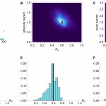
Fig. 1: Simulation results with mean serial interval λ=6 days and R0=0.6.
We simulated 200 different time series with R0 of 0.6 and a three step spillover hazard (Fig. 1A). We assumed that λ, the serial interval for infections (the average time from onset of a primary case to onset of a resulting secondary case), was 6 days (results for λ=3 are shown in Figure 2). Ideally, we would be able to measure – via virological market surveillance or otherwise – the change in the relative spillover hazard over time, leaving just two unknowns: R0 and the absolute magnitude of the spillover hazard. Fig. 1B shows that if we assumed the amplitudes and timings of the steps in the spillover hazard were known, our estimates of R0 were tightly constrained around the true value (Fig. 1E). With current surveillance practices it is likely that far less about the spillover hazard will be known. However, if the risk of transmission from animals is decreased by culling or market closure, this date is often reported12. Therefore we modelled a known drop in spillover hazard date (±7 days), but with nothing else known about the shape or magnitude of the hazard (Fig. 1C). Even in this scenario, we obtained unbiased estimates of R0, although the posterior distributions had higher variance than before (Fig. 1F). In contrast, if we had no information whatsoever about the shape and magnitude of the spillover hazard, we obtained a diffuse posterior distribution, with an apparently biased median value for R0 (Fig. 1D).
Results from inference using simulated time series with R0 =0.6 and mean serial interval λ=3. (A) Time series generated by model. (B) Joint posterior distribution for R0 and absolute spillover hazard from model inference when timing and relative amplitude of spillover hazard are known. (C) Joint posterior distribution for R0 and peak spillover hazard when amplitude and timings of the spillover hazard steps are unknown but the hazard drop date is known. (D) Histogram of estimated value of R0 from model inference using 200 different simulated time series, when neither amplitude nor timings of the spillover hazard steps are known. (E) Histogram of estimated value of R0 when relative amplitude and timings of the spillover hazard steps are known. (F) Histogram of estimated value of R0 when amplitude and timings of the spillover hazard steps are unknown but the hazard drop date is known.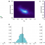
Fig. 2: Simulation results when mean serial interval λ=3.
When secondary cases are generated using a negative binomial distribution with mean equal to R0, and overdispersion parameter 0.1, but inference is performed assuming a Poisson offspring distribution, our estimates for R0 are below the true value (Fig. 3). However, even when the offspring distribution is mis-specified in this way, it is still possible to detect a signature of human-to-human transmission from onset data.
Results from inference using simulated time series with R0=0.6 and λ=6, with a negative binomial offspring distribution in simulations, and Poisson distribution in the inference model. (A) Histogram of estimated value of R0 from model inference using 200 different simulated time series, when neither amplitude nor timings of the spillover hazard steps are known. (B) Histogram of estimated value of R0 when relative amplitude and timings of the spillover hazard steps are known. (C) Histogram of estimated value of R0 when amplitude and timings of the spillover hazard steps are unknown but the hazard drop date is known.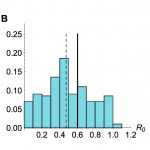
Fig. 3: Sensitivity to mis-specification of offspring distribution
Our model also appears to be insensitive to functional mis-specification of the spillover hazard function, so long as the timing of the drop in hazard is known. In order to examine the sensitivity of our estimates to a mis-specified hazard function, we generated 200 time series using an exponential growth of hazard from spillover exposure and fitted a step-wise spillover hazard function in our analysis (Fig. 4A). Taking the median estimate of R0 from the posterior distributions of the model fits, we found that even with this mis-specification we obtained an unbiased estimate of R0 (Figs. 4B–C).
Model inference when simulated spillover hazard depends on an exponential function, and inference model uses a step function. (A) Representative run when R0 =0.25 and λ=3. Blue points, simulated time series; green line, hazard function in the case generation model. (B) Histogram of median posterior distribution for R0 for 200 time series generated with λ=3. Black line shows true value of R0 =0.25; dashed line, median of inferred values. (C) Histogram of median posterior distribution for R0 for 200 such time series with λ=6.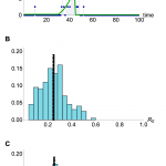
Fig. 4: Sensitivity to mis-specification of hazard function
To test how well the model estimated the proportion of cases that arose from human-human transmission, we simulated 200 time series and recorded whether each case came from an animal-human or human-human source. Fig. 5A shows that the model generally provides good estimates of the proportion of human-human cases, and generates underestimates more often than overestimates. Fig. 5B shows that when simulated secondary cases are overdispersed, there is more variation in estimates of the proportion of human-human transmission. However, the inferred and true values are still strongly correlated: in both cases the Pearson correlation coefficient is >0.8 (p<0.0001).
(A) Comparison of inferred proportion of cases resulting from human-human transmission and actual proportion, for 200 simulated timeseries, using a Poisson offspring distribution. (B) Comparison of inferred human-human cases and actual proportion when offspring distribution is negative binomial with shape parameter 0.1.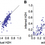
Fig. 5: Inference of proportion of human-human transmission
Influenza A/H7N9 in China
Applying our methods to data from the recent outbreak of influenza A/H7N9 in China, with spillover resulting from exposure to poultry in live bird markets, we found support for the presence of human-to-human transmission, but no evidence that R0 was near the critical value of one. First we calibrated the animal exposure portion of the model in the absence of human-to-human transmission, setting R0=0 and estimating a stepwise hazard with arbitrarily many steps. This framework contains the saturated likelihood model: with a step for every day, we obtain the highest possible probability for the data. However, only a few steps were required for a parsimonious model of animal-to-human-only infections: using the Bayesian Information Criterion (BIC), we see that the models with three or four steps have substantially more support than other hazard functions across Shanghai, Zhejiang and Jiangsu (Table 1). Therefore we used a three step function in the rest of our analysis. Next, we added human-to-human transmission to the spillover model with a three step hazard function and known date for a decrease in hazard (in this instance, the market closure date). Based on cluster data available at the time of the outbreak13, we first assumed λ=9.6 days. Table 1 shows that the model with human-to-human transmission had more support than the animal-to-human-only model for Shanghai and Jiangsu, with both models having similar support for Zhejiang.
Region
Model
Likelihood
Parameters
BIC
Shanghai
2 step
-51.7
3
115.8
3 step
-40.7
5
102.3
4 step
-39.8
7
108.6
5 step
-37.5
9
112.5
6 step
-39.5
11
124.8
7 step
-37.5
13
129.1
Exponential
-41.4
5
103.5
Log-normal
-38.9
7
106.9
Gamma
-39
7
107.1
3 step with H2H
-38
6
100.9
Jiangsu
2 step
-39.6
3
91.8
3 step
-36.4
5
93.7
4 step
-35.3
7
99.8
5 step
-36.1
9
109.9
6 step
-36.4
11
118.9
7 step
-36.9
13
128.3
Exponential
-39.7
5
100.3
Log-normal
-35.8
7
101
Gamma
-36.8
7
103
3 step with H2H
-33
6
91.1
Zhejiang
2 step
-82.8
3
178.2
3 step
-48.1
5
117.2
4 step
-44.4
7
118.3
5 step
-43.5
9
124.9
6 step
-46.1
11
138.4
7 step
-44.6
13
143.9
Exponential
-48.9
5
118.9
Log-normal
-47.9
7
125.2
Gamma
-48
7
125.5
3 step with H2H
-46.9
6
119.1
In all three datasets, the estimate of R0 is well below one and the 95% credible interval around the estimate always excluded one (Table 2). There was evidence of heterogeneity in R0 between these three outbreaks, with two having very similar posterior densities: Shanghai – median 0.19 (95% credible interval 0.01–0.49), and Jiangsu 0.29 (0.03-0.73); and one with support only for much lower values of R0: Zhejiang 0.03 (0.00–0.22).
Region
λ
R0 estimate
Shanghai
3
0.39 (0.02-0.90)
6
0.29 (0.04-0.66)
9.6
0.19 (0.01-0.49)
Jiangsu
3
0.32 (0.02-0.78)
6
0.22 (0.01-0.58)
9.6
0.29 (0.03-0.73)
Zhejiang
3
0.26 (0.00-0.69)
6
0.11 (0.00-0.37)
9.6
0.03 (0.00-0.22)
Figures 6A–C show the posterior distributions for R0, the timing of all other changes in the spillover hazard and the amplitude of the spillover hazard. Despite using only case onset data from publicly available sources, these values are consistent with recently published estimates for R0 based on non-public data obtained during subsequent investigations by China CDC14, which were not available at the time of the outbreak.
Posterior estimates for spillover hazard (in this case resulting from live bird markets) and R0 for influenza A/H7N9 in China, assuming a mean serial interval λ=9.6. (A) Case incidence for Shanghai and the spillover hazard from the best fitting model with market and human-to-human hazard: black dots, observed H7N9 cases; red shaded region, posterior distribution for amplitude of the spillover hazard. Inset: Posterior distribution for R0 in Shanghai. (B) Case incidence for Jiangsu and inferred spillover hazard in best fitting model. (C) Case incidence for Zhejiang and inferred spillover hazard in best fitting model. (D) Estimated number of cases resulting from human-to-human transmission in different regions. Black points, total observed onsets; blue points, estimated non-index cases (with error bars representing 95% credible interval).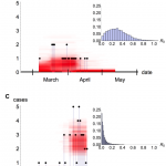
Fig. 6: Estimates for R0 and spillover hazard for A/H7N9 in China
We were also able to estimate the number of observed non-index human cases that resulted from human-to-human transmission (Table 3). Overall, for these three outbreaks, we estimated that 13% (1%–32%) of observed cases arose from human-to-human transmission. The relative patterns in our estimates for R0 and our finding that R0 is below one were unaffected if we instead assumed a smaller serial interval15,16, one of 6 days rather than 9.6 days (Table 2). However, a serial interval of 3 days does increase the estimate of R0 in Zhejiang.
Region
Observed onsets
λ
Non-index cases (95% credible interval)
Shanghai
29
3
8.5 (1.0-22.0)
6
5.9 (0.6-10.5)
9.6
6.9 (0.9-10.7)
Jiangsu
23
3
8.2 (0.9-14.9)
6
5.7 (0.38 -14.6)
9.6
4.4 (1.1-11.8)
Zhejiang
46
3
10.6 (1.4-25.5)
6
3.0 (0.13-22.0)
9.6
1.5 (0.1-6.5)
There has been some speculation that not all cases of influenza A/H7N9 were reported17, however our method produced reliable estimates for R0 even if simulated time series were subject to partial reporting. We considered time series with a mean of 33 observed cases (the average number of observed cases with known onset across the three regions of China we examined), with only 1% or 25% of actual cases observed (Fig. 7).
Histograms of estimated value of R0 from model inference with simulated time series when only timing of drop in spillover hazard known. Market parameters are chosen so that a mean of 33 cases are observed, regardless of reporting rate. 200 different time series were simulated. Each value in the histogram is calculated as the median of the posterior distribution for R0. Solid lines, R0 = 0.6 in the simulated data; dashed line, median of inferred values. Top row, serial interval is 3 days; middle row, 6 days; bottom row, 9.6 days. (A), (B) and (C) All cases observed. (D), (E) and (F) only 25% of cases observed. (G), (H) and (I) Only 1% of cases observed.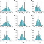
Fig. 7: Sensitivity to under-reporting when drop in hazard known
As was the case with full reporting, the R0 estimates were improved when more information about the hazard function was known (Fig. 8). Although underreporting is a common problem in outbreaks for multiple reasons, these results suggest that our framework could be used reliably even when the true extent of the outbreak is unknown, assuming that cases are reported with a constant probability over time.
Histograms of estimated value of R0 from model inference simulated time series when relative amplitude and timings of spillover hazard known. Market parameters are chosen so that a mean of 33 cases are observed, regardless of reporting rate. 200 different time series were simulated. Each value in the histogram is calculated as the median of the posterior distribution for R0. Solid lines, R0 = 0.6 in the simulated data. Top row, serial interval is 3 days; middle row, 6 days; bottom row, 9.6 days. (A), (B) and (C) All cases observed. (D), (E) and (F) only 25% of cases observed. (G), (H) and (I) Only 1% of cases observed.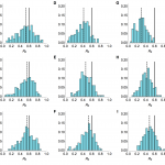
Fig. 8: Sensitivity to under-reporting when shape of hazard known
Emergence of a human transmissible strain
Should similar outbreaks occur in future with R0 > 1, these methods could be valuable in real time to generate the earliest possible evidence of sustained human-to-human transmission. Using a simulated time series with R0 = 1.05 (Fig. 9A), and assuming only the timing of drop in spillover hazard is known, we found our estimate of R0 approached the true value once the spillover hazard decreased, although the credible interval still included many values below one (Fig. 9B). In contrast, if the shape of the spillover hazard – but not the overall amplitude – was known, we obtained useful information about R0, and hence the presence of sustained human-to-human transmission, much earlier (Fig. 9C).
(A) Simulated time series, with cases as blue points and spillover hazard function given by green line. R0 = 1.05 and λ = 6. (B) Real time estimate of R0 when only the timing of drop in spillover hazard was known. Thick blue line, inferred estimate of R0 at that point in time; blue shaded region, 95% credible interval; dashed line, true value of R0. (C) Real time estimate of R0 when shape of the spillover hazard but not the overall amplitude was known.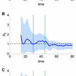
Fig. 9: Estimation of R0 in real time
Discussion
The statistical framework presented here would have substantial value during future outbreaks so long as the timing of drops in hazard are known. Also, if direct evidence of the parametric form of the spillover hazard function over time could be obtained, these methods would provide even more accurate results. With a sufficiently long case time series, repeated simulation and parameter fitting suggests that our model produces unbiased estimates of the basic reproductive number, R0. This is the case even when there is underreporting of cases and when the spillover hazard function is mis-specified as a step function when simulated with exponential growth. We were also able to recover parameters when data were simulated using an overdispersed offspring distribution, and inferred under the assumption of Poisson distributed secondary cases.
Our method adds to the currently available statistical toolkit for analyzing spillover infections. Previous studies have obtained estimates for R0 using data about household-based cases (influenza A/H5N118 and A/H7N719), or by utilizing knowledge that some cases were of animal origin and others were not (influenza A/H3N2v20, influenza A/H5N121 and monkeypox22). Using our model, it is possible to detect a signature of human-to-human transmission for a spillover infection from only the time series of overall clinical incidence.
There are some limitations to the framework and results we have presented. Firstly, we were not able to jointly estimate either the mean or variance of the serial interval distribution for human-to-human infections. Rather, we assumed a value using the best currently available evidence and then tested the sensitivity of key results to changes in that value. Also, we used only publicly available data; additional evidence has become available since 2013 and has confirmed our estimates14. Our reliance on only onset data and not outbreak investigation data can be viewed as a strength: case counts by day of onset are often the earliest data public health decision makers in both local and remote populations have access to when making rapid assessments of risk during a spillover event. Despite these limitations, our formulation adds substantial additional insight to the time series of new cases.
We found evidence that around 13% of observed cases in the three largest clusters of influenza A/H7N9 in China in 2013 resulted from human-to-human transmission, rather than from spillover exposure (this increased to 15% when we assumed a serial interval of 6 rather than 9.6 days). This contrasts with the five potential cases of human-to human-transmission reported out of a total of 136 cases23,24, suggesting that a greater number of human-to-human cases may have been confirmed if additional data on each case’s potential for exposure had been available. It is interesting that the peak of our posterior estimates for R0 in Shanghai and Jiangsu (Figs. 6A–B) is above zero, but for the slightly later epidemic in Zhejiang there is no evidence that R0 is significantly greater than zero (Fig. 6C). These differences in R0 posteriors could be explained by a number of hypotheses. It could be that changes in behaviour – perhaps as a reaction to mass media reports – reduced transmission by the time the Zhejiang outbreak started. Alternatively, differences in human population structure and density, as well as the distribution of markets and bird movements, could have affected the dynamics of the infection in different regions.
The framework we present has substantial potential value for public health. First, the approach can be applied to any outbreak of a spillover infection similar to influenza A, and gives a useful upper bound for R0 consistent with the observed onset data. Second, the results illustrate how being able to characterise the variation in spillover hazard over time can permit accurate estimates of R0 from relatively small outbreaks. For example, to characterise the hazard from avian influenza in poultry markets, weekly random samples could be taken and stored from sentinel markets. In the event of a nearby outbreak of human cases, stored samples could be tested and the temporal variation in spillover risk estimated independent of the incidence of human cases. If this approach were combined with routine sequencing of human isolates, it is possible that fitness increases in the virus could be observed prior to the virus crossing the critical threshold of R0 equal to one.
Author contributions
AJK, HLM and SR designed the study and wrote the paper. AJK and HLM performed the study. AJK, HLM, AP, CF, MDVK, CAD and SR analyzed the data. AJK and HLM contributed equally to the work.
Competing Interests
The authors have declared that no competing interests exist.
Acknowledgements
We thank Neil Ferguson and Simon Cauchemez for useful discussion.References
- Anderson RM, Fraser C, Ghani AC, Donnelly CA, Riley S, Ferguson NM, Leung GM, Lam TH, Hedley AJ. Epidemiology, transmission dynamics and control of SARS: the 2002-2003 epidemic. Philos Trans R Soc Lond B Biol Sci. 2004 Jul 29;359(1447):1091-105. PubMed PMID:15306395.
- Mills CE, Robins JM, Lipsitch M. Transmissibility of 1918 pandemic influenza. Nature. 2004 Dec 16;432(7019):904-6. PubMed PMID:15602562.
- Viboud C, Miller M, Olson D, Osterholm M, Simonsen L. Preliminary Estimates of Mortality and Years of Life Lost Associated with the 2009 A/H1N1 Pandemic in the US and Comparison with Past Influenza Seasons. PLoS Curr. 2010 Mar 20;2:RRN1153. PubMed PMID:20352125.
- Lloyd-Smith JO, George D, Pepin KM, Pitzer VE, Pulliam JR, Dobson AP, Hudson PJ, Grenfell BT. Epidemic dynamics at the human-animal interface. Science. 2009 Dec 4;326(5958):1362-7. PubMed PMID:19965751.
- Jones KE, Patel NG, Levy MA, Storeygard A, Balk D, Gittleman JL, Daszak P. Global trends in emerging infectious diseases. Nature. 2008 Feb 21;451(7181):990-3. PubMed PMID:18288193.
- Cauchemez S, Van Kerkhove MD, Riley S, Donnelly CA, Fraser C, Ferguson NM. Transmission scenarios for Middle East Respiratory Syndrome Coronavirus (MERS-CoV) and how to tell them apart. Euro Surveill. 2013 Jun 13;18(24). PubMed PMID:23787162.
- Cowling BJ, Jin L, Lau EH, Liao Q, Wu P, Jiang H, Tsang TK, Zheng J, Fang VJ, Chang Z, Ni MY, Zhang Q, Ip DK, Yu J, Li Y, Wang L, Tu W, Meng L, Wu JT, Luo H, Li Q, Shu Y, Li Z, Feng Z, Yang W, Wang Y, Leung GM, Yu H. Comparative epidemiology of human infections with avian influenza A H7N9 and H5N1 viruses in China: a population-based study of laboratory-confirmed cases. Lancet. 2013 Jul 13;382(9887):129-37. PubMed PMID:23803488.
- Wallinga J, Teunis P. Different epidemic curves for severe acute respiratory syndrome reveal similar impacts of control measures. Am J Epidemiol. 2004 Sep 15;160(6):509-16. PubMed PMID:15353409.
- White LF, Pagano M. A likelihood-based method for real-time estimation of the serial interval and reproductive number of an epidemic. Stat Med. 2008 Jul 20;27(16):2999-3016. PubMed PMID:18058829.
- Heesterbeek JA. A brief history of R0 and a recipe for its calculation. Acta Biotheor. 2002;50(3):189-204. PubMed PMID:12211331.
- Murhekar M, Arima Y, Horby P, Vandemaele KA, Vong S, Zijian F, Lee CK, Li A. Avian influenza A(H7N9) and the closure of live bird markets. Western Pac Surveill Response J. 2013 Apr-Jun;4(2):4-7. PubMed PMID:24015364.
- Yu H, Wu JT, Cowling BJ, Liao Q, Fang VJ, Zhou S, Wu P, Zhou H, Lau EH, Guo D, Ni MY, Peng Z, Feng L, Jiang H, Luo H, Li Q, Feng Z, Wang Y, Yang W, Leung GM. Effect of closure of live poultry markets on poultry-to-person transmission of avian influenza A H7N9 virus: an ecological study. Lancet. 2013 Oct 30. PubMed PMID:24183056.
- Li Q, Zhou L, Zhou M, Chen Z, Li F, Wu H, Xiang N, Chen E, Tang F, Wang D, Meng L, Hong Z, Tu W, Cao Y, Li L, Ding F, Liu B, Wang M, Xie R, Gao R, Li X, Bai T, Zou S, He J, Hu J, Xu Y, Chai C, Wang S, Gao Y, Jin L, Zhang Y, Luo H, Yu H, Gao L, Pang X, Liu G, Shu Y, Yang W, Uyeki TM, Wang Y, Wu F, Feng Z. Preliminary Report: Epidemiology of the Avian Influenza A (H7N9) Outbreak in China. N Engl J Med. 2013 Apr 24. PubMed PMID:23614499.
- Chowell G, Simonsen L, Towers S, Miller MA, Viboud C. Transmission potential of influenza A/H7N9, February to May 2013, China. BMC Med. 2013 Oct 2;11:214. PubMed PMID:24083506.
- Chen Y, Liang W, Yang S, Wu N, Gao H, Sheng J, Yao H, Wo J, Fang Q, Cui D, Li Y, Yao X, Zhang Y, Wu H, Zheng S, Diao H, Xia S, Zhang Y, Chan KH, Tsoi HW, Teng JL, Song W, Wang P, Lau SY, Zheng M, Chan JF, To KK, Chen H, Li L, Yuen KY. Human infections with the emerging avian influenza A H7N9 virus from wet market poultry: clinical analysis and characterisation of viral genome. Lancet. 2013 Jun 1;381(9881):1916-25. PubMed PMID:23623390.
- Gao HN, Lu HZ, Cao B, Du B, Shang H, Gan JH, Lu SH, Yang YD, Fang Q, Shen YZ, Xi XM, Gu Q, Zhou XM, Qu HP, Yan Z, Li FM, Zhao W, Gao ZC, Wang GF, Ruan LX, Wang WH, Ye J, Cao HF, Li XW, Zhang WH, Fang XC, He J, Liang WF, Xie J, Zeng M, Wu XZ, Li J, Xia Q, Jin ZC, Chen Q, Tang C, Zhang ZY, Hou BM, Feng ZX, Sheng JF, Zhong NS, Li LJ. Clinical findings in 111 cases of influenza A (H7N9) virus infection. N Engl J Med. 2013 Jun 13;368(24):2277-85. PubMed PMID:23697469.
- Yu H, Cowling BJ, Feng L, Lau EH, Liao Q, Tsang TK, Peng Z, Wu P, Liu F, Fang VJ, Zhang H, Li M, Zeng L, Xu Z, Li Z, Luo H, Li Q, Feng Z, Cao B, Yang W, Wu JT, Wang Y, Leung GM. Human infection with avian influenza A H7N9 virus: an assessment of clinical severity. Lancet. 2013 Jul 13;382(9887):138-45. PubMed PMID:23803487.
- Yang Y, Halloran ME, Sugimoto JD, Longini IM Jr. Detecting human-to-human transmission of avian influenza A (H5N1). Emerg Infect Dis. 2007 Sep;13(9):1348-53. PubMed PMID:18252106.
- van Boven M, Koopmans M, Du Ry van Beest Holle M, Meijer A, Klinkenberg D, Donnelly CA, Heesterbeek HJ. Detecting emerging transmissibility of avian influenza virus in human households. PLoS Comput Biol. 2007 Jul;3(7):e145. PubMed PMID:17676981.
- Cauchemez S, Epperson S, Biggerstaff M, Swerdlow D, Finelli L, Ferguson NM. Using routine surveillance data to estimate the epidemic potential of emerging zoonoses: application to the emergence of US swine origin influenza A H3N2v virus. PLoS Med. 2013;10(3):e1001399. PubMed PMID:23472057.
- Ferguson NM, Fraser C, Donnelly CA, Ghani AC, Anderson RM. Public health. Public health risk from the avian H5N1 influenza epidemic. Science. 2004 May 14;304(5673):968-9. PubMed PMID:15143265.
- Blumberg S, Lloyd-Smith JO. Inference of R(0) and transmission heterogeneity from the size distribution of stuttering chains. PLoS Comput Biol. 2013;9(5):e1002993. PubMed PMID:23658504.
- Qi X, Qian YH, Bao CJ, Guo XL, Cui LB, Tang FY, Ji H, Huang Y, Cai PQ, Lu B, Xu K, Shi C, Zhu FC, Zhou MH, Wang H. Probable person to person transmission of novel avian influenza A (H7N9) virus in Eastern China, 2013: epidemiological investigation. BMJ. 2013 Aug 6;347:f4752. PubMed PMID:23920350.
- Li Q, Zhou L, Zhou M, Chen Z, Li F, Wu H, Xiang N, Chen E, Tang F, Wang D, Meng L, Hong Z, Tu W, Cao Y, Li L, Ding F, Liu B, Wang M, Xie R, Gao R, Li X, Bai T, Zou S, He J, Hu J, Xu Y, Chai C, Wang S, Gao Y, Jin L, Zhang Y, Luo H, Yu H, He J, Li Q, Wang X, Gao L, Pang X, Liu G, Yan Y, Yuan H, Shu Y, Yang W, Wang Y, Wu F, Uyeki TM, Feng Z. Epidemiology of human infections with avian influenza A(H7N9) virus in China. N Engl J Med. 2014 Feb 6;370(6):520-32. PubMed PMID:23614499.

Leave a Comment
You must be logged in to post a comment.