Abstract
Background: The evolution of antiviral drug resistance during influenza pandemics has created widespread concern. Use of antiviral drugs is a main contributor to the evolution of drug-resistant strains. Moreover, there are recent examples of influenza viruses acquiring drug resistance seemingly without incurring a fitness penalty that reduces their transmission rate. This creates the possibility of strategic (game theoretical) interaction between jurisdictions making decisions about use of antiviral drug stockpiles.
Methods: We developed and analyzed a 2-player 2-strategy game theoretical model. Each ‘player’ (an authority in a health jurisdiction) can choose to treat with antiviral drugs at a low rate or a high rate. High treatment rates are more likely to cause emergence of a drug-resistant strain, and once a drug-resistant strain has evolved, it can spread between the two jurisdictions. We determine the Nash equilibria of the game.
Results: We show that there is a coordination game between the jurisdictions, where both players choosing a low treatment rate, or both choosing a high treatment rate, are the only stable outcomes. The socially optimal outcome occurs if both players cooperate by choosing a low treatment rate, thereby avoiding generating drug-resistant mutants. However, such cooperation may fail to materialize if the jurisdictions are closely connected through travel; if the drug-resistant mutant is tolerated (not seen as undesirable); or if the antiviral drug has partial efficacy against transmission of the drug-resistant strain.
Conclusions: Inter-jurisdictional cooperation could be essential during a severe influenza pandemic, but we know little about how jurisdictions will interact in a scenario where highly pathogenic, drug-resistant mutant strains are able to transmit as effectively as non-resistant strains. Therefore, strategic multi-population interactions during influenza pandemics should be further studied.
Funding Statement
This work was supported by a research grant to Chris Bauch from the Canadian Institutes of Health Research. The funders had no role in the design, analysis, writing, or decision to submit the manuscript for publication.Background
The 1918-1919 H1N1 influenza pandemic was a deadly event, killing an estimated 50-100 million people worldwide1. Subsequent pandemics occurred in 1957 and 1968, and the World Health Organization confirmed the beginning of another pandemic on June 11, 20092,3. Vaccines were not available until the middle of the 2009 pandemic in many populations, and the problem of limited vaccine availability may occur in future pandemics until vaccine production technologies change. Thus, at the start of a pandemic, antiviral drugs may be the only available pharmaceutical intervention. Therefore, the frequent emergence of drug-resistant viruses has raised serious concerns.
Acquiring a mutation often entails tradeoffs, such that a strain that acquires drug resistance also suffers a fitness penalty (e.g., a reduced transmission rate). There is a rich literature on the implications of tradeoffs for pathogen strain structure and transmission dynamics4,5. In the context of influenza subtype H1N1, the H274Y mutation weakens binding of the drug oseltamivir to viral neuraminidase (NA) enzyme, by reducing the amount of NA that is available at the cell surface6. However, this also has the effect of reducing the fitness of the virus, since NA is necessary for the virus to be released from the host cell. As a result, acquisition of the H274Y mutation without any secondary compensatory mutations can reduce the evolutionary fitness of the virus6. Drug resistance is less problematic when mutants are less transmissible than original strain (for instance, as a result of a fitness penalty), since the mutants can be outcompeted by the original strain in community-level transmission. Indeed, most early oseltamivir-resistant strains appeared to have reduced transmissibility and infectivity, compared to their non-resistant progenitors7.
However, more recently, influenza A (H1N1)pdm09 viruses have been increasingly capable of acquiring the H275Y mutation that confers oseltamivir-resistance, without suffering a fitness penalty, thanks to secondary mutations6,8. In the 2007-2008 influenza season in Europe, oseltamivir-resistant influenza A (H1N1) with the H275Y mutation emerged and was observed to spread widely even in absence of widespread antiviral drug usage, suggesting that the mutants competed well with the resistant strains already in circulation6,9 . Drug resistance due to oseltamivir usuage also emerged more quickly than in pre-pandemic strains7,9,10. Additionally, it appears that influenza A (H7N9) viruses are also capable of acquiring oseltamivir resistance without suffering a fitness penalty11. (However these viruses have not yet evolved the ability to transmit from person-to-person in a sustainable way12,13.)
The emergence of oseltamivir-resistant influenza viruses that are as transmissible as their non-resistant progenitors has implications for how jurisdictions decide upon antiviral drug strategies during a pandemic. Mathematical models have been used to determine optimal antiviral drug use strategies that minimize the emergence and/or spread of antiviral drug resistant strains in a single jurisdiction14,15,16,17. When drug resistance confers a fitness penalty, single-jurisdiction approaches are adequate, since the less transmissible mutant will be outcompeted by the original strain in another jurisdiction that has chosen to practice limited antiviral drug use. However, when evolution of drug resistance fails to cause a reduced transmission rate, a careful policy of restricting antiviral drug use to limit the emergence of resistant strains may not be helpful to a jurisdiction that is connected to another jurisdiction through travel: the jurisdiction practicing limited antiviral drug usage remains susceptible to importing the drug-resistant strain from the other jurisdiction practicing high rates of antiviral drug use. Without a fitness penalty, the drug-resistant strain can spread freely in both jurisdictions, even though only one jurisdiction generated the mutant strain.
If the socially optimal approach is to restrict treatment only to the severest infections and thereby avoid or limit the emergence of drug resistance, then two jurisdictions may cooperate with one another by both using antiviral drugs at a low rate. However, if one jurisdiction is treating at a high rate and thereby generating many drug-resistant mutants, then there is little incentive for the other jurisdiction to continue treating at a low rate, if importation of the resistant strain from the other jurisdiction seems likely. Instead, the jurisdiction may want to treat at a high rate as well, in which case both jurisdictions end up adopting the socially suboptimal strategy of using antiviral drugs at a high rate. This strategic aspect of antiviral drug use policy between health jurisdictions has not yet received much attention in the public health literature, to our knowledge.
Game theory is the formal study of decision-making where several players must make choices that potentially affect the payoffs of the other players. A Nash equilibrium is a state where no player can increase his or her payoff by unilaterally switching to a different strategy. More specifically, suppose that player i choosing strategy ai gets a payoff ui(ai, aj) when the other player j chooses strategy aj . A strategy ai* is a strict Nash equilibrium for player i if we have ui(ai*,aj)>ui(a-i, aj) for every other player i strategy a-i≠ai* and for every possible strategy aj adopted by player j26. Hence, there is no incentive for any player to change their strategy and we generally expect that rational players will choose Nash equilibrium strategies (convergence issues aside). In this paper we will only consider conditions for strict Nash equilibria, although we will refer simply to Nash equilibria throughout for brevity. The application of classical game theory to individual human behaviour has been criticized for its assumption that each player ‘rationally’ maximizes his or her own payoff without considering the impact of their decisions on the well-being of other players. In real populations, social processes may make this assumption untenable18. However, it may be a better description of how countries, regions, or municipalities interact with one another in a severe pandemic.
Some previous multi-population models have also incorporated human behaviour19,20. These are based on compartmental epidemiological models, and focus on paediatric infectious disease. Other models explore the effect of individual adaptive decision-making on the epidemiology of infectious diseases21,22, or address the emergence and control measures of antiviral drug resistance in a single population 14,15, but do not consider strategic interactions between multiple populations. Models of strategic inter-jurisdictional antiviral drug usage during an influenza pandemic appear to be rare, although approaches have been developed for other types of infectious diseases31,32.
In this Background section we have provided intuition for why antiviral drug use decisions may create strategic interactions when drug resistance fails to confer a fitness penalty. In the remainder of this paper we develop and analyze a formal game theoretical model of how two health jurisdictions choose antiviral drug use strategies in a situation where the drug resistant strain can travel between the jurisdictions. This allows us to gain insight regarding: when such strategic interactions are likely to become important, what form the strategic interactions will take place, and when such interactions are more likely to result in socially suboptimal (i.e. non-Pareto optimal) outcomes. Our objective was to illustrate the wide range of possible outcomes that may occur in such situations, and to show how the outcomes may depend on epidemiological, geographical, and perceptual factors. Our objective was not to generate quantitatively correct predictions about strategic interactions in specific, real-world populations for specific influenza strains. In such cases, where models are intended to serve didactic purposes rather than predictive purposes, a simpler model is often preferable to a complicated model23. Hence, we opt to use simple game theoretical model based on fixed payoff matrices, rather than a more sophisticated dynamic evolutionary game theoretical model combined with a disease transmission model. Although this creates some limitations in terms of model interpretation, it also enables us to more easily discuss and classify different possible strategic outcomes under different circumstances.
Methods
We developed a symmetric 2-player, 2-strategy game where payoffs are derived from a posteriori epidemiological and antiviral drug assumptions. Each player is an authority making decisions that affect their health jurisdiction and can choose to either treat at a low rate L, which we interpret to mean using antiviral drugs only for the severest infections, or to treat at a high rate H, which we interpret to mean using antiviral drugs for both severe and non-severe infections, and possibly also for prophylaxis. The payoffs depend on the final epidemic size, which is a parameter. Consider a given “focal” player for which we are determining payoffs based on epidemic outcomes in their focal jurisdiction, depending partly on what the “other” player in charge of the other jurisdiction does. We let R(x, y) denote the epidemic final size (the number of recovered individuals at the end of the epidemic) of the regular strain in the focal jurisdiction,
where x is the treatment level in the focal jurisdiction, y is the treatment level in the other jurisdiction, κ is the final size of the regular strain if both players treat at a low rate, η is the final size if the focal player treats at a low rate and the other treats at a high rate, and δ is the final size if the focal player treats at a high rate.
The final size δ when the focal player treats at a high rate does not depend on the strategy of the other player because we assume that only a small proportion of individuals travel between the jurisdictions, hence case imports from the other player’s jurisdiction are only a small part of the total incidence of infection in the focal jurisdiction. We expect δ< κ, since a player that treats at a high rate will reduce the transmission of the regular strain, and hence will have a smaller final epidemic size of the regular strain. We expect δ< η for the same reasons. Generally, we expect η< κ, since the other player treating at a high rate instead of a low rate will create some small incremental benefit for the focal jurisdiction, by reducing the number of case imports of the regular strain. However, this effect is small if travel is small, such as for populations connected primarily through airplane travel, and so one could equally well assume κ= η for simplicity, when travel is infrequent. In summary, δ< η ≤ κ, which simplifies to δ< η= κ by our assumption.
Similarly, we let Rm(x, y) denote the epidemic final size of the drug-resistant strain in the focal jurisdiction, where Rm(x, y) is given by
where x and y denote treatment levels for the focal player and the other player respectively, β is the final size of the drug-resistant strain if the focal player treats at a high rate, and γ is the final size of the drug-resistant strain if the focal player treats at a low rate and the other player treats at a high rate.
We assume that there is no emergence of drug-resistant influenza virus if both jurisdictions treat at a low rate, hence Rm (L, L)=0. If the focal jurisdiction treats at a high rate, then drug-resistant mutants are created, and the final epidemic size of the drug-resistant strain is β. Again β does not depend on the strategy of the other player, since the focal player is already creating a large number of drug-resistant mutants through liberal use of antiviral drugs, and a few more case imports will not contribute much to the final size of the drug resistant strain. However, if the focal player treats at a low rate and the other player treats at a high rate, then the focal jurisdiction experiences a non-trivial final size of the drug-resistant strain, denoted γ. γ is affected by the degree of isolation between the jurisdictions. The greater the isolation (i.e. the fewer travels between jurisdictions), the less the mutant strain emerging from a high treatment jurisdiction impacts a low treatment jurisdiction.
One possibility is that β > γ, because a high number of mutants are generated in jurisdiction 1 due to the high treatment level. This is more likely to occur when the jurisdictions are more isolated. Conversely, we may have that β < γ, especially when the jurisdictions are closer together: the focal jurisdiction experiences an inflow of drug-resistant strains from the other jurisdiction, and the mutants can spread effectively in the focal jurisdiction once they have become established. However, because the focal jurisdiction is not using antiviral drugs (which are assumed to have partial efficacy against the drug-resistant strains) at a high rate, the final size of the mutant strain is very large. The relationship between β and γ thus depends on the exact nature of travel connections, how much less effective the drug is in controlling the drug resistant strain, and how transmissible the resistant strain is compared to the regular strain. We explore these two cases.
The payoff P of a focal player that adopts treatment rate x when the other player treats at the rate y is
where M is a constant representing health payoff in absence of a pandemic (we can set M=0 without loss of generality) and α is the weighting factor that determines control priorities.In a focal jurisdiction that treats at rate x while the other jurisdiction treats at rate y, R and Rm are the final sizes of recovered individuals from the regular and mutant strains, respectively. We generally assume α< 0.5, meaning that the jurisdictions consider a case of mutant strain influenza to be more undesirable than a case of regular strain influenza.
We furthermore assume P(H) ≡ P(H, H)= P(H, L) where P(H) is the payoff of a focal player playing H. The rationale for this assumption is that when case imports of the regular strain are rare, the final size of the regular strain in a jurisdiction is determined primarily by the actions of the player controlling that jurisdiction. (The case where P(H, H)≠ P(H, L) is briefly described in the Discussion section.) By assuming P(H, H)= P(H, L) (i.e., if a player treats at high level, its payoff is independent of the other player’s strategy), the payoffs for the three possible outcomes for equation 1 and equation 2 are:
The payoff matrix of this game appears in Figure 1. Although the relationships between the three entries of the payoff matrix depend on the assumed values β, γ, κ, η, δ, and α, we generally expect that P(L, L)> P(H, H)= P(H, L)> P(L, H) for an undesirable drug-resistant strain (see discussion at beginning of methods). Thus, if both jurisdictions treat at a low level, they both have a high payoff. If both jurisdictions treat at high levels, both have medium payoffs. In the case where one has a high treatment level and the other a low treatment level, the high treatment level jurisdiction has a medium payoff and the low treatment level jurisdiction a low payoff.
Baseline parameters
We set parameter values according to published epidemiological literature whenever possible, allowing us to specify plausible values for κ, η, δ (Table 1) that also satisfied the inequalities described in the Methods section24,25. The other parameters β, γ, and α were varied during our analysis.
Table 1. Parameters, values, and descriptions: R and Rm are the final sizes of the regular and mutant strains in focal jurisdiction.
Results
Conditions for multiple versus single Nash Equilibria
Coordination games are a class of games with multiple pure strategy Nash equilibria26. The players can choose one Nash equilibrium or the other Nash equilibrium depending on process that may lead them naturally to one or the other. A coordination game can be yielded by a payoff matrix which we use here, with the likely relationships between P(L, L), P(L, H), P(H, L), and P(H, H) described in the Methods section (Figure 1). If both players adopt high treatment levels (H) then they both will have medium payoffs, P(H, H)≡ m; if both players have low treatment levels (L) and thereby avoid generating drug-resistant mutants, then both players will have high payoffs, P(L, L)≡ h; if focal player has low treatment rate and other player has high treatment rate then focal player will have low payoff, P(L, H)≡ l (since focal player treated at a low rate to avoid generating mutant strains, but was infected by mutant strains anyway due to the high treatment rate of other player ) and other player has medium payoff, P(H, L)≡ m. We assume h> m> l, so the game has exactly two Nash equilibria at (H, H) and (L, L). Thus, it is an unbalanced coordination game where the players could adopt either (H, H) or (L, L) depending on how they coordinate their actions. We note that very different (non-coordination) games may emerge if h> m> l does not hold.
Figure 1. The payoff matrix for the focal player. The focal player’s strategies are to treat at a high rate (‘H’, row 1), or at a low rate (‘L’, row 2) while the other player’s strategy is also to treat at a high rate (‘H’, column 1) or a low rate (‘L’, column 2). Parameters l, m and h represent low, medium, and high payoffs respectively. P(x,y) is the payoff to the focal player when the focal player plays x and the other player plays y. Other parameter values are defined in the Methods and Results sections.
According to this argument, the focal point in this game (i.e. the Nash equilibrium that we expect the players to adopt) is at (L, L) which both jurisdiction tend to choose in the absence of communication. There is a natural tendency to choose the (L, L) strategy, not only because of higher payoffs but also because of the likely temporal development of the pandemic. Initially, the number of infections will be low and hence the players might start out playing an “L” strategy to begin with. If that is the case, they would simply stay at (L, L) as the pandemic unfolds. However, if α is very small, such as might occur due to a mutant that is perceived as particularly severe, the players may `panic’ and converge to the (H, H) strategy.
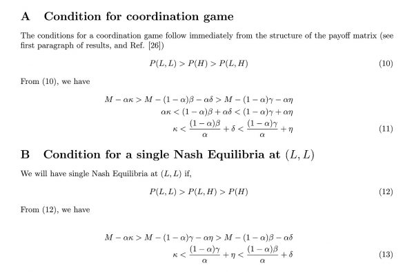
However, a closer investigation of the dependence of strategic outcomes on the epidemiological parameters β, γ, κ, η, δ, and α reveal a more subtle picture with a greater range of possible outcomes than this approximate argument can provide (see Table 2 for summary). It can be shown (Appendix A) that a coordination game emerges if
Since κ > δ, the leftmost inequality in inequality (5) is dependent upon the magnitude of (1 – α)β/α, which is decreasing in α. Therefore, the leftmost inequality may be satisfied when the mutant strain is sufficiently undesirable (i.e., α is sufficiently small). Regarding the rightmost inequality in inequality (5), η > δ, yet the relationship between β and γ is dependent upon the degree of connectedness of the jurisdictions. When the jurisdictions are highly connected, we have γ > β and thus the rightmost inequality is trivially satisfied. However, more isolated jurisdictions with β > γ satisfy the rightmost inequality for sufficiently high α. In summary, coordination games exist when mutant strains are sufficiently undesirable, and also when jurisdictions are sufficiently connected. However, for isolated jurisdictions, inequality (5) might also be satisfied by an intermediate value of α.
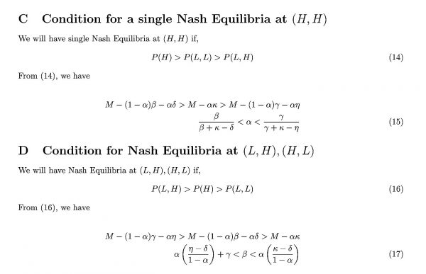
It can be shown (Appendix B) that a single Nash equilibrium at (L, L) occurs when
Since we assume that κ = η, the left hand inequality in (6) is trivially satisfied. However, the right hand inequality depends upon the relation of β and γ. Opposite to the coordination game case, the right hand inequality is never satisfied when the jurisdictions are highly connected, since η > δ and γ > β. However, if the jurisdictions are isolated such that β > γ, then the inequality may still be satisfied if the mutant strain is sufficiently undesirable.
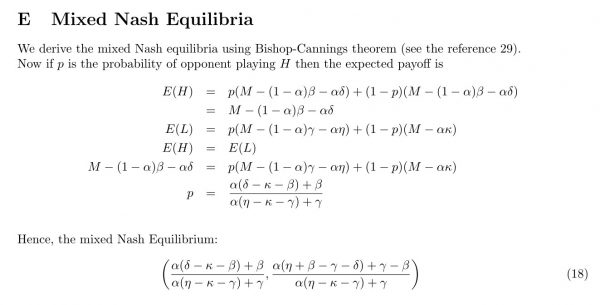
The condition for (H, H) to be a Nash equilibrium (see Appendix C) is:
In general, this equation is satisfied when β is sufficiently small and γ is sufficiently large, corresponding to the situation where the jurisdictions are closely connected. Also, it requires that α takes on an intermediate value, which encourages players to use more antiviral drugs since the mutant strain is less undesirable. We furthermore note that the rightmost inequality is satisfied if κ < η (which cannot occur under our assumptions), and if κ ≥ η, it can be satisfied when α is sufficiently small and when γ is sufficiently large.
It is also possible that (L, H), (H, L) occurs as a Nash equilibrium (see Appendix D), when:
In this case, it can be shown that
Hence, the player treating at a low level is free-riding on the benefits provided by the player treating at a high level. At these parameter values, the player adopting H provides benefits to the player adopting L by reducing case imports of infections to their jurisdiction. In practice, this could occur if one player first moves from a lower to a higher treatment rate early during the pandemic, due to the relation P(H, L) > P(L, L). However, once that player has switched to high treatment, the fact that P(L, H) > P(H, H) means that the player who is slower to switch strategies has no incentive to also switch to high treatment rates. Hence, the Nash equilibrium is (L, H), (H, L). However, since κ ≈ η and γ > 0 are reasonable assumptions, meaning that the leftmost term in inequality (8) will generally exceed the rightmost term and thus violate the inequality, we expect this outcome to be rare.
Finally, this game admits a mixed strategy Nash equilibrium which is found using the Bishop-Cannings theorem29. A mixed strategy is one in which a player plays his available pure strategies with a given probability. If p is the probability of opponent playing H then it can be shown (Appendix E) that the mixed Nash Equilibrium p* is
Parameter planes showing how these equilibrium states depend on model parameters are useful for better understanding these results. For a given value of the final size of the mutant strain if a player treats at a high rate (β), a less undesirable mutant strain (higher α) shifts the outcome from a single Nash equilibrium at (L, L) to two Nash equilibria at (H, H) and (L, L) (Figure 2). This occurs because a less `scary’ or dangerous mutant strain reduces the incentive to maintain low treatment levels. If the final size of the mutant strain for a player treating at a low rate while the other player is treating at a high rate (γ) is higher, there is a similar effect of turning (H, H) into a second Nash equilibrium: increasing γ increases the strength of externalities, since the other player treating at a higher rate has a larger impact on the focal player treating at a lower rate. An increase in γ may occur due to stronger travel connections between the two jurisdictions, for instance. Finally, we observe from Figure 2 that decreasing β, the final size of the mutant strain for a player treating at a high rate, also causes (H, H) to become a second Nash equilibria. This occurs because a reduced final size of the mutant strain under high treatment rates incentivizes high treatment rates, since it corresponds to the (often unrealistic) situation where widespread use of the drug significantly reduces the final size of the drug-resistance strain.
Table 2. Conditions for different equilibria.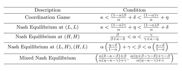
Figure 2. α-γ parameter plane. The α-γ parameter plane divided into regions containing one or two Nash Equilibria for various β values. The region above each line contains two Nash Equilibria at (L, L) and (H, H) while the region below each line contains single Nash equilibria at (L, L).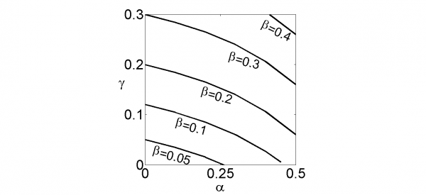
Parameter planes of β versus γ for various values of α show a wider range of possible outcomes, especially when α is larger (Figure 3). Here we again observe that low values of β (an unrealistic region of parameter space corresponding to a low final size of mutant infections under high treatment rates) or high values of γ (corresponding to stronger externalities due to closer travel connections) correspond to a region of parameter space where both (H, H) and (L, L) are Nash equilibria. In contrast, when β is large and/or γ is small, (L, L) is the only Nash equilibrium. Moreover, as α increases, corresponding to a less undesirable mutant strain, the region where (H, H) is the sole Nash equilibrium appears and begins to expand. This occurs because when α is larger, generating mutants is less of a concern and hence higher treatment rates are acceptable. As α increases, a region with two Nash equilibrium (L, H) and (H, L) also appears, but it occupies a very small region of the parameter space (see also Figure 4, which shows a blown-up version of Figure 3f). Our model does not account for time spent in transit, such as time spent in an airplane, or commuting via public transit or automobile. This might have an impact on our results if jurisdictions are connected by plane travel and symptom screening stations are set up at airport arrival terminals. However, it would not have an impact for jurisdictions connected primarily through public transit or automobile, for which screening is impractical.
Figure 3. β-γ parameter plane. The β-γ parameter plane divided into various regions depending on number and type of Nash equilibrium they contain, for α=0.01 (a), 0.1 (b), 0.2 (c), 0.3 (d), 0.4 (e) and 0.5 (f). Nash equilibria are indicated by (H, H), etc.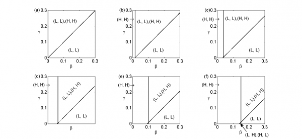
Figure 4. β-γ parameter plane. The β-γ parameter plane divided into various regions depending on number and type of Nash equilibrium they contain, for α=0.5. Nash equilibria are indicated by (H, H), etc. This figure is equivalent to Figure 3f.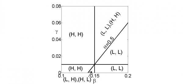
In summary, the best scenario for an outcome of (L, L) where both players adopt low treatment levels occurs when: the jurisdictions are not strongly connected through travel (low γ), high levels of treatment would result in a high final size of infections by mutant strains (high β), and/or the mutant strain is highly undesirable (low α). Most importantly, jurisdictions with close travel ties (low γ) and with the potential for mutants that do not respond to the antiviral drug (large β) are more subject to outcomes such as (H, H) due to externalities, and if α is also small, then outcomes could be socially suboptimal (i.e. non-Pareto optimal) since both jurisdictions end up treating at high rate due to strategic considerations.
Stackelberg Equilibria
The temporal development of events that occur during a real influenza pandemic could change the strategic nature of antiviral usage. For instance, the pandemic strain would first emerge in a single jurisdiction that might have to make decisions about antiviral usage before other jurisdictions that are presently virus-free.
The concept of a Stackelberg equilibrium is useful under these circumstances of a sequential game27. In a Stackelberg equilibrium, one player acts as a leader and the other as a follower. The leader adopts a strategy, taking into account the follower’s optimal response strategy. It differs from the Nash equilibrium in which players act simultaneously. We will denote focal jurisdiction as the leader, where the pandemic starts, and other jurisdiction as the follower.
Under conditions where (L,L) or (H,H) are the only Nash Equilibria in the case of simultaneous play, then sequential play does not alter the predictions of our analysis. However, for the conditions that lead to a coordination game in the simultaneous case (P(L, L) > P(H) > P(L, H)) the outcome of sequential play differs from the simultaneous case. Sequential play permits the leader to direct the outcome to the (L,L) equilibrium, since the leader can surmise that the follower will choose H if it chooses H, and L if it chooses L. Thus, the leader will choose L, since P(L,L) > P(H).
Figure 5. Tree diagram for Stackelberg equilibria. Tree diagram for Stackelberg equilibria where RL and RF are the rates adopted by the leader and the follower respectively. Also. l, m, and h are low, medium, and high payoffs.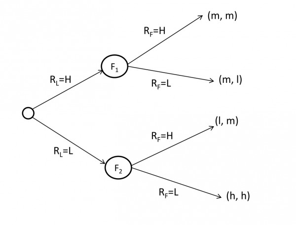
Under conditions where we have the equilibria (L,H) and (H,L) in the simultaneous case, sequential play benefits the leader. If the leader chooses L, then the follower will choose H. And, if the leader chooses H, then the follower will choose L. Thus, we arrive at one of the two Nash Equilibria. Since P(L,H) > P(H), the leader will choose L, and thus force the follower to take the lesser payoff, H. Therefore, sequential play benefits the leader.
Discussion
Here we developed a two-player game of strategic interactions in antiviral usage during an influenza pandemic. The model highlights the possibility for externalities to develop, if a drug resistant influenza strain is as transmissible as the non-resistant variety. Under such circumstances, it is possible for a socially suboptimal Nash equilibrium to develop where both players use antiviral influenza drugs at a high rate, when the socially optimal behaviour is actually for both players to treat at a low rate. This occurs because players may opt to treat at a high rate, knowing that drug-resistant mutants will emerge and be imported to their jurisdiction anyway, due to high antiviral drug usage in the other jurisdictions. In this scenario, there is a Nash equilibrium at (L, L) where both jurisdictions treat at a low rate, and a socially suboptimal equilibrium at (H, H) where both jurisdictions treat at a high rate. We found that such a scenario is more likely when the two jurisdictions are closely connected through travel (γ is high), since travel connections increase the chances of case importations. A higher travel volume increases the chance that a mutant strain is imported from the other jurisdiction, and therefore increases the likelihood that the jurisdiction will increase its treatment rate in anticipation of receiving mutant strains from the other jurisdiction. Similarly, socially suboptimal Nash equilibria such as (H,H) or coordination games also occur when the mutant strain is tolerated (α is high). This causes the players to be less concerned about generated drug-resistant strains and therefore more likely to choose H. Finally, a socially suboptimal Nash equilibrium could occur if the antiviral drug is effective in reducing the final size of the drug resistant strain (β is low). However, antiviral drugs seem to have little influence on the final size of drug-resistant influenza strains30 and so a situation where β is low may not occur in reality. In summary, a socially suboptimal outcome where two Nash equilibria are possible and player choose the one corresponding to a higher treatment rate occurs if the jurisdictions are closely connected through travel; if the drug-resistant mutant is tolerated (not seen as undesirable); or if the antiviral drug has partial efficacy against the drug-resistant strain.
In the Stackelberg model, in which players play sequentially, we found that conditions for both players to use antiviral drugs at a low rate were weaker (easier to satisfy). Such cases in which the Stackelberg model applies are: when the emergence of a disease is observed in a single jurisdiction, or when the disease is observed in both jurisdictions, but one jurisdiction is able to react faster.
Our model considers an implied stochastic setting where players incur a probability to generate a mutant strain if they treat with antiviral drugs at a high rate. Because of this, when the volume of travel between the populations is sufficiently low, the main impact that a jurisdiction might have on other jurisdictions is if they treat with antiviral drugs at a very high rate, while other jurisdictions treat at a low rate. In that case, the jurisdictions treating at a low rate may receive case imports of mutant strains from the jurisdiction treating at a high rate (P(L, H)≠ P(L, L)), despite their attempts to treat at a low rate to avoid the emergence of antiviral drug resistance. On the other hand, a jurisdiction treating at a high rate is already generating mutant strains and is therefore little affected by other jurisdictions in this respect (P(H,H)=P(H,L)). Naturally, differing assumptions about travel volume or the impact of antiviral drugs on the epidemiology of the drug-resistant strain could change the predictions. Thus, future work could explore this effect through a stochastic, two-patch model.
Like other models, this model has some limitations. Perhaps most importantly, we derive payoffs from a posteriori epidemiological and antiviral drug assumptions. This was intentional, since our objective was to illustrate that the outcomes of strategic interactions in antiviral drug usage between jurisdictions during an influenza pandemic could vary widely depending on epidemiological (β), geographical (γ), and perception of the severity of the mutant strain compared to the resistant strain (α) . However, the drawback of using a posteriori assumptions is that it is difficult to quantify the exact likelihood of various outcomes, or even to quantify the outcomes themselves. For instance, we do not know what value of α real health authorities might adopt. Similarly, although we interpret (H, H) to represent a socially suboptimal outcome where both jurisdictions engage in excessive antiviral drug use, we would need to better quantify the relationship between treatment levels and outcomes (for instance, by using a mechanistic model and/or using real cost estimates) in order to firmly establish this. A further limitation is that we did not capture stochastic events, which are important in the context of drug resistance evolution since mutation events are stochastic. We also assumed that jurisdictions can control stockpiles of drugs and that they may quickly and accurately dispense them during a pandemic. Additionally, this model is not based on an infectious disease transmission model, and thus we could not study any temporal dynamics.
Similarly, predictions might change if the Stackelberg model were changed to a multiple turn game where we alternate between the jurisdictions, giving them the option to increase their treatment levels. Under conditions where P( L , L ) < P( H ) < P( L , H ), both jurisdictions wish for the other to treat at a high level while they treat at a low level. In a repeated game this could result in a so-called Mexican standoff where neither side wishes to treat. However, this leads to the worst case scenario for both jurisdictions, ( L , L ), because of the assumption P( L , L ) < P( H ) < P( L , H ).
The quantities P(H, H) and P(H, L) are in fact only approximately equal when case imports are not too high. Our assumption that P(H, H) = P(H, L) may break under the various circumstances. For instance we could achieve P(H, H) > P(H, L) if the use of the high antiviral treatment level in the other jurisdiction significantly decreases the number of cases that are imported from to the focal jurisdiction, and increases the focal player’s payoff (relative to the case where the other player uses the low treatment level). Alternatively, P(H, H) < P(H, L) could happen if the use of the high treatment level at the other jurisdiction significantly increases the risk of a drug resistant strain arising, and being imported into the focal jurisdiction, and that the spread of such a strain is very costly to the focal jurisdiction. We speculate that these conditions are more likely to arise when the travel rates between the two jurisdictions are very high. It can be shown that we have a coordination game under these circumstances when P(L, L) > P(H, L) and P(H, H) > P(L, H). However, we leave a full exploration of the case P(H, H)≠ P(H, L) to future work.
Other model limitations include lack of heterogeneity in the patient population and patient health status in particular, and the lack of including other drivers of behaviour. For instance, some individuals may have risk factors for severe infection, such as co-infection with HIV or advanced age. Such patients would merit a higher priority for antiviral drug treatment, and the moral imperative to provide treatment for those individuals could modify strategic considerations. To some extent, heterogeneity in patient health status is implicitly accounted for in our model: we allow for a low treatment strategy, but not a zero treatment strategy, because we assume that some individuals will always be treated. However, our assumption that the low treatment strategy will not produce antiviral drug resistance may not apply under all circumstances. Moreover, there may be other consequences of population heterogeneities for strategic interactions that we have not foreseen. It is difficult to know whether such heterogeneities would strengthen or weaken strategic interactions a priori, therefore further research on this topic is needed. Strategic considerations could also be modified by political or economic factors. Political decisions receive input from factors other than strategic considerations, and likewise economic factors could be a strong determinant of antiviral drug use strategies. For instance, many countries simply cannot afford to practice prophylaxis or widespread treatment with antiviral drugs. Similarly, social cohesion could influence decisions and prevent a “rational” Nash equilibrium from materializing, either in favour of higher antiviral drug use, or lower antiviral drug use28. A model with multiple jurisdictions and connected by complex network could also result in very different predictions than our simple two jurisdiction model. Finally, we note that when antiviral drug resistance can emerge de novo–independently of antiviral drug use–the nature of strategic interactions could change significantly, which has implications for predicted outcomes.
We leave it to future work using more realistic models to refine some of the results of our simple model, and determine more precisely the likelihood that strategic factors could become important, and what the corresponding outcomes would be. For now, this initial model shows that strategic interactions could potentially play a role in antiviral drug use decisions, and it calls for further research with more detailed and empirically motivated models.
Conclusion
The model shows how a wide range of outcomes are possible depending on epidemiological, geographical, and perceptual factors in the populations. Externalities caused by travel connections when drug-resistant mutants do not suffer a reduced transmission have the potential to lead both jurisdictions to socially suboptimal states of excessive antiviral drug use. Strategic interactions between jurisdictions during an influenza pandemic should be further studied.
List of abbreviations
L: treat at a low rate
H: treat at a high rate
l: low payoff
m: medium payoff
h: high payoff
WHO: World Health Organization
HIV: Human Immunodeficiency Virus
Corresponding Author
Please contact Kamal Jnawali at [email protected]
Competing Interest Statement
The authors have declared that no competing interests exist.
Data Availability Statement
All data appearing in the manuscript were generated directly from the equations in the manuscript. No new simulation code or epidemiological data were generated as a result of this research.
Appendices
References
- Morens, D. M., & Fauci, A. S. (2007). The 1918 influenza pandemic: insights for the 21st century. Journal of Infectious Diseases, 195(7), 1018-1028.
- Chan, M. (2009). World now at the start of 2009 influenza pandemic. World Health Organization.
Reference Link - Pandemic (H1N1) 2009 - update 81. World Health Organization.
Reference Link - Bowers, R. G., Boots, M., & Begon, M. (1994). Life-history trade-offs and the evolution of pathogen resistance: competition between host strains. Proceedings of the Royal Society of London B: Biological Sciences, 257(1350), 247-253.
- Day, T. (2003). Virulence evolution and the timing of disease life-history events. Trends in Ecology & Evolution, 18(3), 113-118.
- Bloom, J. D., Gong, L. I., & Baltimore, D. (2010). Permissive secondary mutations enable the evolution of influenza oseltamivir resistance. Science, 328(5983), 1272-1275.
- Aoki, F. Y., Boivin, G., & Roberts, N. (2006). Influenza virus susceptibility and resistance to oseltamivir. Antiviral therapy, 12(4 Pt B), 603-616.
- Butler, J., Hooper, K. A., Petrie, S., Lee, R., Maurer-Stroh, S., Reh, L., ... & Leang, S. K. (2014). Estimating the fitness advantage conferred by permissive neuraminidase mutations in recent oseltamivir-resistant A (H1N1) pdm09 influenza viruses. PLoS Pathog, 10(4), e1004065.
- Meijer, A., Lackenby, A., Hungnes, O., Lina, B., Van Der Werf, S., Schweiger, B., ... & Zambon, M. (2009). Oseltamivir-resistant influenza virus A (H1N1), Europe, 2007–08 season.
- Kiso, M., Mitamura, K., Sakai-Tagawa, Y., Shiraishi, K., Kawakami, C., Kimura, K., ... & Kawaoka, Y. (2004). Resistant influenza A viruses in children treated with oseltamivir: descriptive study. The Lancet, 364(9436), 759-765.
- Hai, R., Schmolke, M., Leyva-Grado, V. H., Thangavel, R. R., Margine, I., Jaffe, E. L., ... & Bouvier, N. M. (2013). Influenza A (H7N9) virus gains neuraminidase inhibitor resistance without loss of in vivo virulence or transmissibility. Nature communications, 4.
- Centers for Disease Control and Prevention (CDC. (2013). Emergence of avian influenza A (H7N9) virus causing severe human illness-China, February-April 2013. MMWR. Morbidity and mortality weekly report, 62(18), 366.
- Longini, I. M., Halloran, M. E., Nizam, A., & Yang, Y. (2004). Containing pandemic influenza with antiviral agents. American journal of epidemiology, 159(7), 623-633.
- Chao, D. L., Bloom, J. D., Kochin, B. F., Antia, R., & Longini, I. M. (2012). The global spread of drug-resistant influenza. Journal of The Royal Society Interface, 9(69), 648-656.
- Stilianakis, N. I., Perelson, A. S., & Hayden, F. G. (1998). Emergence of drug resistance during an influenza epidemic: insights from a mathematical model. Journal of Infectious Diseases, 177(4), 863-873.
- Regoes, R. R., & Bonhoeffer, S. (2006). Emergence of drug-resistant influenza virus: population dynamical considerations. science, 312(5772), 389-391.
- Moghadas, S. M., Bowman, C. S., Röst, G., & Wu, J. (2008). Population-wide emergence of antiviral resistance during pandemic influenza. PLoS One, 3(3), e1839.
- Gintis, H. (2009). The bounds of reason: Game theory and the unification of the behavioral sciences. Princeton University Press.
- Montopoli, L., Bhattacharyya, S., & Bauch, C. T. (2009). The free rider problem in vaccination policy and implications for global eradication of infectious diseases: a two-country game dynamic model. Canadian Applied Mathematics Quarterly, 17(2), 317-338.
- Bauch, C. T. (2005). Imitation dynamics predict vaccinating behaviour. Proceedings of the Royal Society of London B: Biological Sciences, 272(1573), 1669-1675.
- Funk, S., Salathé, M., & Jansen, V. A. (2010). Modelling the influence of human behaviour on the spread of infectious diseases: a review. Journal of the Royal Society Interface, 7(50), 1247-1256.
- Jones, J. H., & Salathe, M. (2009). Early assessment of anxiety and behavioral response to novel swine-origin influenza A (H1N1). PLoS one, 4(12), e8032.
- May, R. M. (2004). Uses and abuses of mathematics in biology. Science, 303(5659), 790-793.
- Gani, R., Hughes, H., Fleming, D., Griffin, T., Medlock, J., & Leach, S. (2005). Potential impact of antiviral drug use during influenza pandemic. Emerg Infect Dis, 11(9), 1355-1362.
- Nichol, K. L., Lind, A., Margolis, K. L., Murdoch, M., McFadden, R., Hauge, M., ... & Drake, M. (1995). The effectiveness of vaccination against influenza in healthy, working adults. New England Journal of Medicine, 333(14), 889-893.
- Osborne, M. J. (2004). An introduction to game theory (Vol. 3, No. 3). New York: Oxford University Press.
- Hamilton, J. H., & Slutsky, S. M. (1990). Endogenous timing in duopoly games: Stackelberg or Cournot equilibria. Games and Economic Behavior, 2(1), 29-46.
- Oraby, T., Thampi, V., & Bauch, C. T. (2014). The influence of social norms on the dynamics of vaccinating behaviour for paediatric infectious diseases. Proceedings of the Royal Society of London B: Biological Sciences, 281(1780), 20133172.
- Bishop, D. T., and Chris Cannings. "A generalized war of attrition." Journal of Theoretical Biology 70.1 (1978): 85-124.
- Lipsitch, Marc, et al. "Antiviral resistance and the control of pandemic influenza." PLoS Med 4.1 (2007): e15.
- Klepac, P., Megiddo, I., Grenfell, B. T., & Laxminarayan, R. (2016). Self-enforcing regional vaccination agreements. Journal of The Royal Society Interface, 13(114), 20150907.
- Montopoli, L., Bhattacharyya, S., & Bauch, C. T. (2009). The free rider problem in vaccination policy and implications for global eradication of infectious diseases: a two-country game dynamic model. Canadian Applied Mathematics Quarterly, 17(2), 317-338.


Leave a Comment
You must be logged in to post a comment.